Applied Fieldwork
Qualitative vs Quantative Data
Qualitative data is data that cannot be measured, such as field notes or sketches.
Quantitative data is data that can be measured, such as the width of a beach or dimensions of a stone.
Quantitative data is data that can be measured, such as the width of a beach or dimensions of a stone.

Primary vs Secondary Data Collection
Primary data is data that you collect yourself, such as measuring the length of a beach.
Secondary data is data that you get from a secondary source, such as getting the length of a beach from a map.
Secondary data is data that you get from a secondary source, such as getting the length of a beach from a map.

Random data vs Stratified Data vs Systematic Data
Random sampling is used where the study area is the same throughout. In a flat grassy field, you could assume that the environmental conditions do not change within the meadow, it doesn’t matter whereabouts within the area you take your samples from. In urban investigations, you might use random sampling if, for example, you are assessing a small number of sites in one particular housing estate for environmental quality.
Random sampling can be used to choose spots or areas as sites to sample. It is vitally important that you do not choose sample sites yourself, as this will introduce bias. Random sampling is achieved by generating two random numbers (from a random number table or a scientific calculator) and using them as co-ordinates. For a small area, such as a field, you could lay two 20m tape measures on the ground and use the co-ordinates to place a quadrat. For an urban area, you could use the co-ordinates to generate Ordnance Survey grid references.
Random sampling should be free from bias. But it may be difficult to obtain a truly representative sample. The number of samples that you take (the sampling size) is important.
Systematic sampling is used when the study area includes an environmental gradient. With an environmental gradient you would expect a variable to change in a regular manner as you move away from the start of your survey e.g. the depth of the river as you move further away from the source. You could sample along a line (e.g. at 10 equally spaced points on 3km of a river's course to investigate downstream changes in a river or every 20m along a line running inland in a sand dune system) or in every grid square within a defined area (e.g. within every 100m x 100m grid square within a small area for flood hazard mapping). Sample points should be evenly spaced or distributed.
Systematic sampling is quick and easy to do. But it is easy to miss variation. For example, if you are investigating downstream changes in a river by choosing equally spaced samples, you may not easily be able to pick out the effect of tributaries joining the river. If you are investigating a sand dune system, widely spaced intervals may mean that you miss some variations in vegetation, such as small dune slacks. It is important to consider a suitable distance between your intervals so as not to miss a rapid change (eg sand dune succession). The number of samples that you take (the sampling size) is important and the area that you complete your sample in.
Stratified sampling is used when the study area includes significantly different parts (also known as subsets). You should make sure that the number of samples taken is representative of the importance of each subset within the total population. In a rivers investigation into the effect of stream ordering on discharge, a stratified sample would be to choose sites where the two river segments of the same order join. In a sand dune investigation, a stratified sample would be to choose to sample where on dunes of different ages rather than at equally spaced intervals. In a drainage basin that is 30% clay and 70% sandstone, you may choose to collect data from 3 sites on clay and 7 sites on sandstone. Stratified sampling should overcome the problem with missing variation that might arise with systematic sampling, but it can be difficult to get background data to allow you to apply stratified sampling appropriately.
What is a Transect?
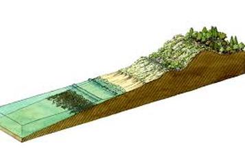
A transect is a line following a route along which a survey or observations are made. The transect is an important geographic tool for studying changes in human and/or physical characteristics from one place to another, such as from the sea to a path that runs along the beach.
Data Collection on Field Trip to Highcliffe
On the year 10 trip to highcliffe, we gathered a variety of different kinds of data. To start with, we drew a transect from the sea to the path that ran parallel to it. We then split this transect into sections of 3 meters from which we gathered our data.
To start with, we measured the angle of the beach. To do this we dug a meter stick into the sand at each 3 meter intersection. We then used a gun clinometer to measure the angle between the top of each meter stick (see image below). After collecting this data we used all of the measurements to work out an average angle. This was good because it was systematic data, all measured in the same way. However, a gun clinometer is subject to many human errors, because it requires a human to aim it.
To start with, we measured the angle of the beach. To do this we dug a meter stick into the sand at each 3 meter intersection. We then used a gun clinometer to measure the angle between the top of each meter stick (see image below). After collecting this data we used all of the measurements to work out an average angle. This was good because it was systematic data, all measured in the same way. However, a gun clinometer is subject to many human errors, because it requires a human to aim it.
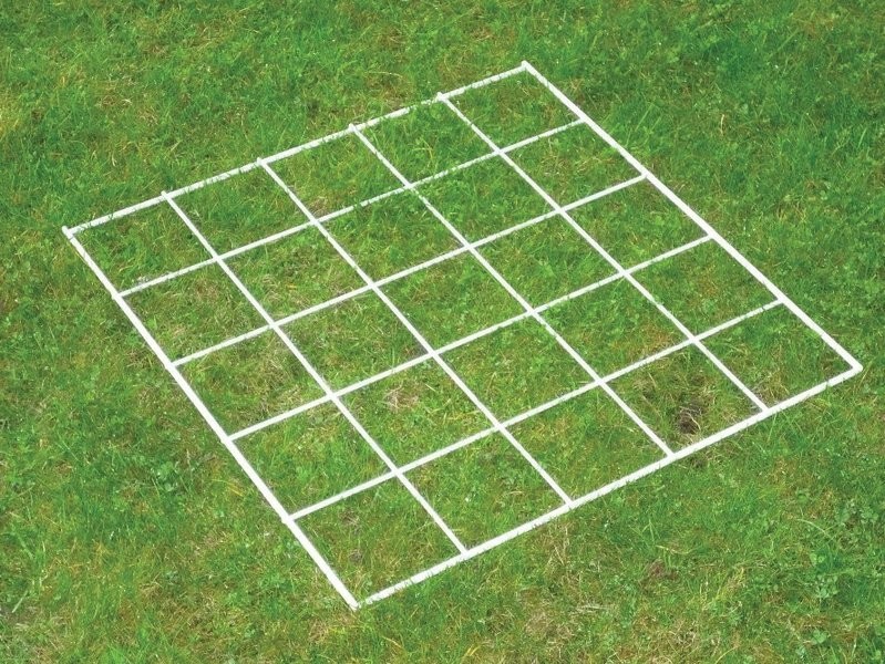
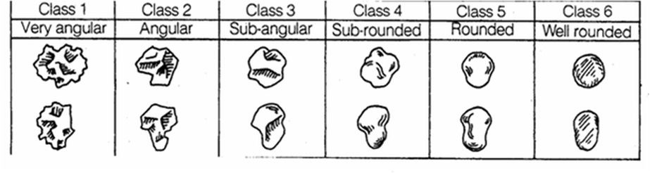
After that we measured the dimensions and volume of stones from each section, working out an average for each 3 meter section. To measure the dimensions we used calipers (see picture below) to measure 3 stones (which we selected systematically using a quadrat) then worked out an average this is good because it meant that we measured all the stones in the same way however, we only measured them in cm which is not very accurate. With the 3 stones we then sorted them into classes using the table below (this is not very accurate because it is subjective to opinion). To measure the volume we filled a jug with water to a certain point, we then added 10 randomly selected pebbles to the jug, taking the original reading away, we divided by 10 to find an average volume.

|
|
null hypothesis for highcliffe field trip
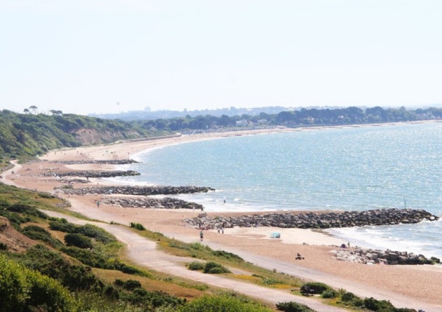
Long shore drift does not go from west to east. This was disproved when we discovered that the waves were coming in from the west. As shown in the picture below.
|
Transects of the beach at highcliffe
These transects however prove the null hypothesis as correct. As the beach got thicker at the west end, meaning that the shingle was getting deposited at the west instead of the beach.We can see this as transect 2 (which was at the west) had a width of 54m and a maximum height of 7m. Transect 5 however (which was at the east) had a width of 30m and a maximum height of 4.5m, this means that the long shore drift was traveling from east to west as more sediment was deposited at the west end. Transect 1 was an anomaly as it did not follow the pattern of the others.
